Block 1 · 12:00–12:50 · Measurement Chain and Sensor Fundamentals
Sensors, Actuators, GPIO, and Serial Interfaces
4.1 The Measurement Chain
A sensor system converts a physical, chemical, or biological phenomenon into usable information. The chain may contain a sensing element, excitation, analog front end, filtering, amplification, analog-to-digital conversion, compensation, digital processing, calibration coefficients, communication, timestamping, and application interpretation.
An analog-output sensor leaves conversion and much validation to the host system. A digital sensor may return compensated engineering units. A smart sensor may estimate orientation, recognize objects, reject invalid echoes, or report diagnostics. More onboard processing reduces host workload but can hide assumptions and failure modes inside undocumented firmware.
Physical quantity | Sensing element | Conditioning and ADC | ||
Timestamped data and decision | Digital / industrial interface | Compensation, filtering, calibration |
Figure 4.1. A practical measurement chain. The sensor package may contain only the sensing element or nearly the entire chain.
4.2 Reading Sensor Specifications Correctly
Sensor selection begins with the measurand and operating conditions, not the connector or available library. The following terms answer different questions.
| Property | Meaning and practical consequence |
|---|---|
| Range | Interval over which performance is specified. A device may output values beyond it without those values being trustworthy. |
| Span | Difference between upper and lower range limits. |
| Sensitivity | Change in output per change in input, such as mV/kPa. High sensitivity does not automatically mean high accuracy. |
| Resolution | Smallest distinguishable or represented change. Digital bit depth gives quantization resolution, not complete system resolution. |
| Accuracy | Closeness to an accepted reference under stated conditions. Specifications may combine offset, gain, nonlinearity, and temperature effects. |
| Precision | Closeness among repeated results. A precise sensor can be consistently wrong. |
| Repeatability | Agreement when the same method and conditions are repeated over a short interval. |
| Reproducibility | Agreement when conditions, operators, instruments, or times change according to a defined procedure. |
| Linearity | Deviation from a chosen straight-line relationship. A nonlinear sensor can still be accurate after valid compensation. |
| Hysteresis | Different output for the same input depending on whether the input approached from above or below. |
| Dead band | Input interval that produces no observable output change. Common in mechanical systems and valves. |
| Property | Meaning and practical consequence |
|---|---|
| Offset and gain error | Constant output shift and scale error, respectively. They require different calibration models. |
| Drift | Output change over time at constant input, caused by aging, contamination, stress, or environment. |
| Noise | Random variation from the sensor, electronics, environment, power, electromagnetic coupling, or quantization. |
| Cross-sensitivity | Response to a quantity other than the intended measurand, such as humidity influence on a gas sensor. |
| Response time | Time required to approach a defined fraction of the final response after an input change. Always check the criterion. |
| Bandwidth | Frequency interval over which dynamic response meets a defined limit. |
| Saturation | Region where increasing input no longer produces a meaningful corresponding output. Saturated data are not simply “large values.” |
| Uncertainty | Quantified doubt associated with the measurement, based on identified contributions and stated coverage. |
Accuracy and resolution are frequently confused. A 16-bit ADC across 3.3 V has a nominal code width near 50 μV, but reference error, front-end noise, sensor tolerance, layout, and calibration may make the usable accuracy far worse. Displaying many decimal places does not create information.
4.3 Static Calibration, Uncertainty, and Traceability
Calibration compares indications with a reference under defined conditions and estimates a relationship. For a linear model,
where x is raw indication and y is the estimated measurand. Calibration does not repair poor placement, hysteresis, saturation, insufficient response time, contamination, or use outside the calibrated range.
For n ≥ 2 repeated observations x₁, …, xₙ, the sample mean and standard deviation are
The mean summarizes the observed level, and the standard deviation describes sample dispersion; neither alone establishes closeness to the reference value. For independent observations from a stationary process, the standard uncertainty of the mean due to repeatability is estimated by s/√n. Correlated samples need a different treatment. Averaging a biased sensor produces a more stable biased result.
An uncertainty budget may include reference uncertainty, repeatability, resolution, calibration fit, temperature, supply variation, mounting, spatial variability, and drift. For a measurement model y = f(x₁, …, xₘ), independent input standard uncertainties are propagated to first order as
Here cᵢ converts the uncertainty of input xᵢ into output units. A direct root-sum-square is appropriate only when the contributions are already expressed as output standard uncertainties. Correlated inputs require covariance terms; strongly nonlinear models may require propagation of full probability distributions. State assumptions, units, and any coverage factor rather than presenting an unjustified percentage [86].
Traceability means that a result can be related to a reference through a documented, unbroken calibration chain with stated uncertainties. A comparison against an uncharacterized second low-cost sensor is a functional check, not necessarily traceable calibration.
4.4 Dynamic Behavior, Response Time, and Saturation
Many sensors behave approximately as a first-order system:
where τ is the time constant and K the steady-state sensitivity. After a step, an ideal first-order response reaches about 63.2% of its final change after one τ, 95% after roughly 3τ, and 99% after roughly 4.6τ.
Response depends on packaging and installation. A protected temperature sensor inside a massive enclosure may be electrically fast but thermally slow. A gas sensor behind a membrane has transport delay. A soil probe may be dominated by contact and spatial heterogeneity. Sampling faster than the physical response does not make the phenomenon respond faster.
Saturation can occur in the sensing element, amplifier, ADC, or onboard algorithm. A rail value may mean true full scale, overrange, power failure, broken wiring, or a numerical limit. Detect repeated exact extrema, quality flags, impossible derivatives, and inconsistency with redundant information. Recovery from chemical, optical, or magnetic saturation may take time even after the stimulus returns to range.
4.5 Sampling, Aliasing, Timing, and Filtering
For ideal reconstruction of a baseband signal band-limited to fmax, sample uniformly at fs > 2fmax. Real systems require an analog anti-alias filter and margin because useful signals and interference are not perfectly band-limited. Once an aliased frequency enters sampled data, a digital filter cannot reconstruct the missing information uniquely.
Sampling rate should follow the physical dynamics and decision requirement. A slowly changing air-temperature sensor may need seconds between useful samples; an IMU used for stabilization may require hundreds of samples per second. Timestamp near acquisition. Record sequence, observation time, receive time, and dropped-sample status where latency matters.
A moving average
reduces some high-frequency variation but adds delay and can smear abrupt events. A first-order exponential filter
is computationally simple but also trades noise reduction for lag. Median filtering can reject isolated spikes but alters signal shape. Filtering must be justified by the noise and application, not used to make an unattractive plot look smooth.
4.6 Representative Sensors for Embedded and Robotic Systems
Table 4.2 is a selection guide, not an endorsement. Exact voltage, address, rate, accuracy, and protocol depend on the breakout board and product revision. A module may add regulators, level shifters, or protocol conversion not present in the sensing IC.
Table 4.2. Examples of sensors commonly encountered with Arduino, Raspberry Pi, ESP32, robotics, and mechatronics.
| Device/type | Measures | Interface | Reality, strengths, and limitations |
|---|---|---|---|
| BME280 | Temperature, relative humidity, pressure | I²C or SPI | Compact environmental sensor with factory coefficients; host software converts raw readings into compensated units. Placement, board heating, enclosure, condensation, and airflow often dominate results. |
| BMP280/BMP390 | Pressure and temperature | I²C or SPI | Useful for pressure and relative altitude trends. Weather and reference pressure limit absolute altitude; it does not measure humidity. |
| SHT3x/SHT4x | Temperature and humidity | I²C | Good digital integration. Condensation, contamination, self-heating, and slow enclosure exchange remain important. |
| DS18B20 | Temperature | 1-Wire | Unique address and several devices on one bus. Cabling, pull-up, conversion time, counterfeit devices, and waterproof-probe construction require attention. |
| DHT11/DHT22 | Temperature and humidity | Proprietary pulse timing | Inexpensive and simple but relatively slow, limited, and timing-sensitive; not a reference instrument. |
| Thermocouple + interface | Temperature difference | Microvolt analog; interface IC via SPI | Wide temperature capability. Needs cold-junction compensation, suitable wire, noise control, and open-circuit detection. |
| PT100/PT1000 RTD | Temperature | Resistance through precision front end | Stable industrial measurement. Lead resistance, excitation self-heating, wiring configuration, and analog design matter. |
| Photoresistor | Light-dependent resistance | Analog divider | Cheap qualitative sensing; nonlinear, variable, temperature-sensitive, and unsuitable for calibrated illuminance without characterization. |
| TSL2591/BH1750 | Light/illuminance-related response | I²C | Digital range control and easier integration. Spectral response and geometry differ from human vision and plant response. |
| Device/type | Measures | Interface | Reality, strengths, and limitations |
|---|---|---|---|
| VL53L0X/VL53L1X | Optical time-of-flight distance | I²C | Compact ranging with onboard timing/processing. Target reflectivity, ambient light, field of view, cover glass, and multipath affect results. |
| TFmini/TF-Luna family | Single-point LiDAR distance and signal strength | UART; some variants I²C | Onboard emitter timing, echo detection, and range estimation reduce host work. Sunlight, dark/angled targets, minimum range, beam divergence, multipath, and update-mode configuration matter. |
| HC-SR04-type ultrasonic | Distance | Trigger/echo pulse | Low cost. Often uses 5 V logic; affected by surface angle, soft targets, temperature, crosstalk, blind zone, and specular echoes. |
| MPU-6050 | 3-axis accelerometer + gyroscope | I²C | Common teaching IMU. Bias, temperature drift, vibration, limited calibration, and module quality limit navigation. |
| ICM-20948/BMI270 | Accelerometer and gyroscope; ICM-20948 also includes a magnetometer | I²C or SPI | Higher-rate inertial sensing. Orientation still requires calibration and fusion; magnetic disturbance is a major practical issue. |
| BNO055/BNO085 class | IMU with onboard fusion | I²C, UART, or SPI depending on product | Outputs orientation estimates and calibration status. Convenient, but internal algorithm assumptions, latency, frame conventions, and magnetic environment must be understood. |
| GNSS module (u-blox class) | Position, velocity, and time | UART, USB, I²C, or SPI depending on module | Onboard radio correlation and navigation solution. Accuracy depends on sky view, antenna, multipath, corrections, constellation, dynamics, and solution status. |
| Quadrature encoder | Shaft/wheel position and speed | A/B digital pulses; optional index | Excellent relative motion feedback. Missed edges, electrical noise, direction convention, mounting, wheel slip, and integer rollover matter. |
| Hall-effect sensor | Magnetic field, speed, proximity, or current | Digital or analog | Contactless and robust; sensitive to magnet geometry, air gap, temperature, and external fields. |
| Load cell + HX711 | Force/weight | Millivolt bridge; module digital clock/data | High sensitivity at low cost. Mechanical mounting, creep, temperature, vibration, excitation, and calibration dominate performance. |
| INA219/INA226 class | Bus voltage and inferred current/power | I²C | Useful power monitoring with programmable conversion. Shunt selection, common-mode range, heating, calibration, and transient bandwidth matter. |
| PIR module | Change in infrared scene | Digital | Low-power motion indication, not object ranging. Detects changes, with dead time and sensitivity to temperature, optics, and placement. |
| Device/type | Measures | Interface | Reality, strengths, and limitations |
|---|---|---|---|
| Capacitive soil-moisture probe | Permittivity-related soil response | Analog, frequency, SDI-12, or digital by model | Correlates with water content only after soil-specific consideration. Salinity, density, temperature, installation, air gaps, and corrosion matter. |
| NDIR CO₂ module | CO₂ concentration | UART, I²C, analog, or Modbus | Onboard optical processing and compensation. Warm-up, pressure, humidity, contamination, drift, and automatic baseline assumptions can bias field data. |
| Electrochemical gas sensor | Gas concentration | Nanoamp/microamp analog via potentiostat | Selective only to a degree; cross-sensitivity, temperature/humidity, aging, zero drift, warm-up, and calibration gas are critical. |
| Camera | Images, indirectly many scene properties | CSI, USB, Ethernet | Very information-rich. Illumination, exposure, optics, calibration, motion blur, bandwidth, privacy, and inference errors dominate. |
| 2D/3D LiDAR | Range scan or point cloud | UART, USB, Ethernet, CAN by product | Direct geometric data with onboard timing. Weather, dust, reflective materials, blind zones, multipath, scan timing, and moving-platform distortion matter. |
| Radar | Range, velocity, angle depending on product | SPI, CAN, UART, or Ethernet | Operates in difficult light and some weather. Interpretation, multipath, interference, resolution, antenna placement, and regulatory constraints matter. |
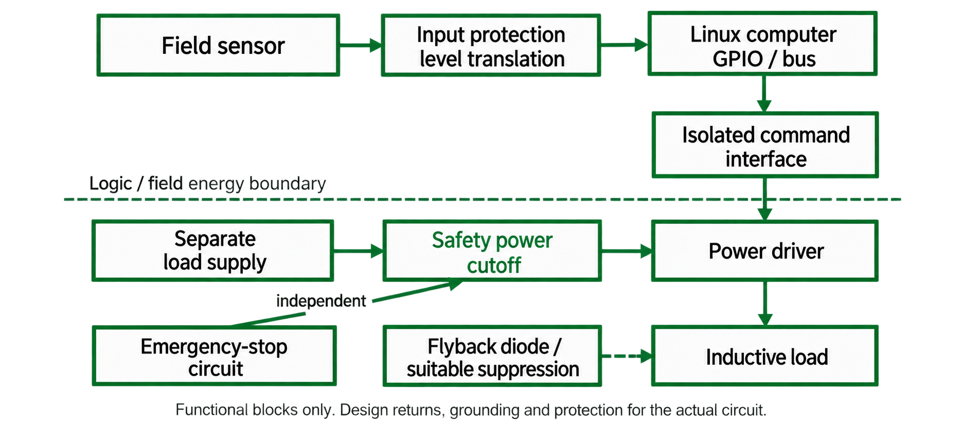
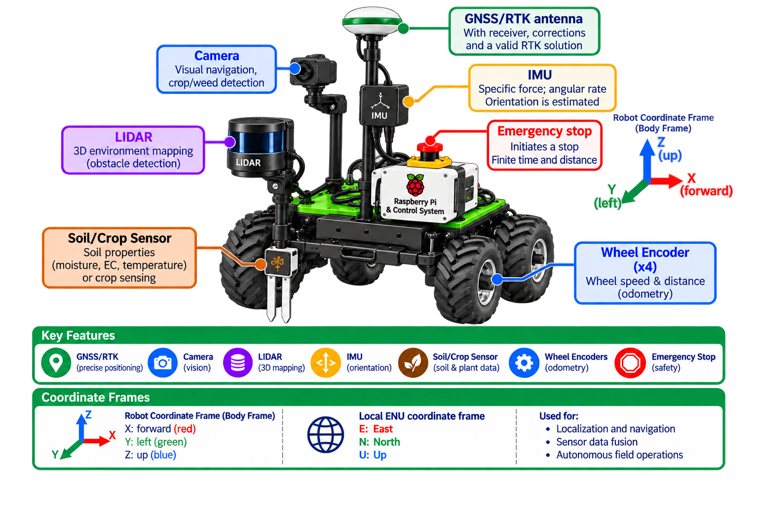
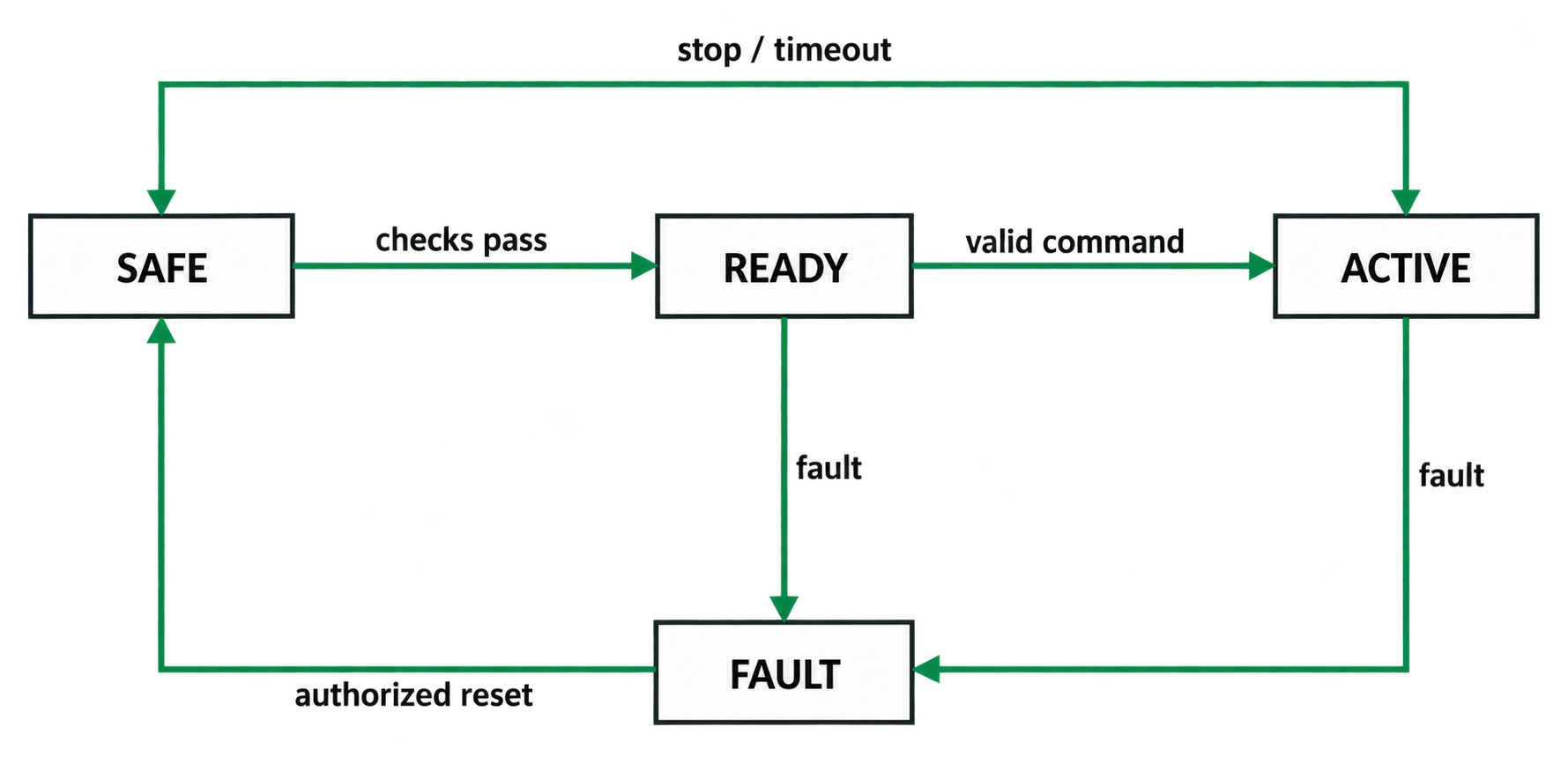 Figure 4.4.